In this post, let’s take a look at the VLOOKUP function, its syntax, and its usage.
How to Use VLOOKUP in Google Sheets
VLOOKUP (Vertical Lookup) is a commonly used function in Google Sheets to search for a specific value from a dataset. As per the name, it searches the column vertically for a key and returns the value of a specific cell.
VLOOKUP Syntax
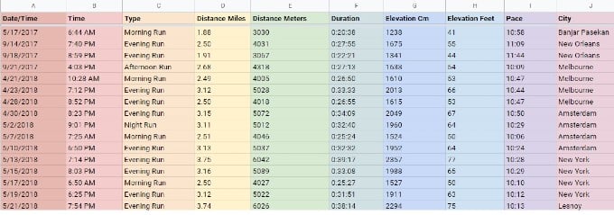
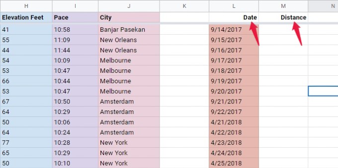
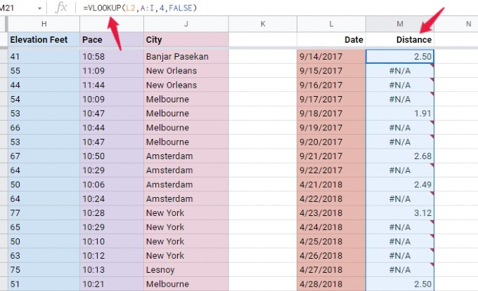
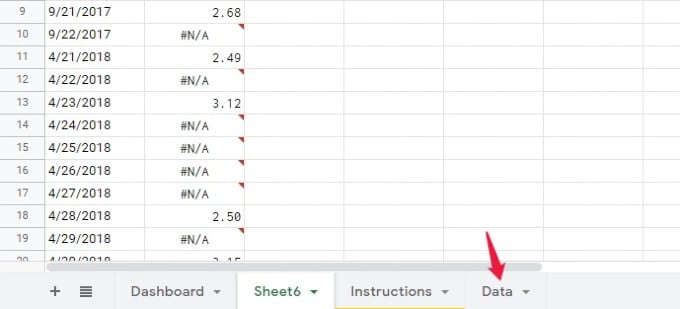
The syntax of the VLOOKUP function is given below: VLOOKUP(search_key, range, index, [is_sorted]) search_key: This field represents the value to search for. It can be a text, number, or alphanumeric. range: Here, you need to specify the range of columns for performing the search. For example, if you mention B:E, then the function will search the columns from B to E. index: This indicates the column index that contains the value returned by the function. is_sorted: It indicates whether the column to be searched is sorted or not. By default, this field is set to TRUE. However, this field is set to FALSE in most cases. Now, let’s try to understand the VLOOKUP function with an example. Let’s imagine you are trying to analyze the running/activity details of someone. And, the Google sheet contains multiple columns like date, time, distance, duration, pace, elevation, city, etc. Let’s say you want to create another table that contains only Date and Distance. Go ahead and add the titles “Date” and “Distance” on columns L and M in the same sheet. Now, you can make use of the VLOOKUP function to get the distance covered on a particular date. VLOOKUP(L2,A:I,4,FALSE) Here, L2 represents the date (search_key) for which the value is returned. A: I (range) indicate the range of columns included in the search. In this example, the fourth Column D contains the distance. Therefore, the value of the index field is set to 4. After entering the formula and pressing ENTER key on your keyboard, you can see that cell M2 contains the distance covered on the date in L2. Likewise, to get the distance for other dates, just drag the cell M2 so that you will get the data on other cells in the column. In case, if the search returns no data, then the cell value will show #N/A. In this example, you can see the value #N/A for all days during which the person has not run.
How to Use VLOOKUP in Multiple Google Sheets
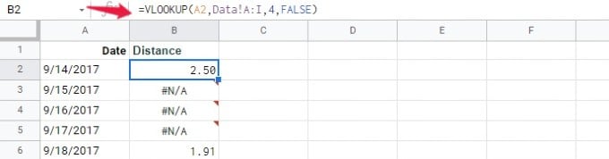
Do you need to create a new table on another sheet in the same document? You can use VLOOKUP function across multiple sheets. For instance, in the above section, the new columns L and M were created in the same sheet. Instead, you can use VLOOKUP function in a new sheet also. Let’s see how to do that. Create a new sheet in your document and add two columns ‘Date’ (A) and ‘Distance’ (B). Now, for every date, we need to get the distance from another sheet titled Data. So, the formula for VLOOKUP will be VLOOKUP(A2,Data!A:I,4,FALSE) As you can see, the formula is very similar to the one explained in the last section. The only difference is Data! which indicates the name of the sheet.
How to Find Partial Match using Wildcards in VLOOKUP
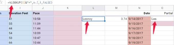
In the above examples, the VLOOKUP function returned a value only if the value in search_key got an exact match. Let’s say you want to find a value in the table that isn’t an exact match, but a partial match. In such scenarios, you can use wildcards. In Google Sheets, you can use three types of wild cards: Asterik(), Question mark(?), Tilde(~). The question mark is used to match for a single character while the asterisk is for any series of characters. . If you need to match an actual question mark or asterisk, then you have to add a tilde (~) before the character. In this example, let’s say you want to find out the distance covered in a particular city. However, you don’t have only the partial name of the city. Now, let’s see how to use the VLOOKUP formula using the wildcard (). VLOOKUP(O2&"*",A:J,1,FALSE) Here, O2 contains the partial search_key (eg. Les). When it is concatenated with the wildcard *, VLOOKUP will search for the data that contains the search_key. (eg. Lesnoy) Next time you are trying to create a new table from an existing table, you can use the VLOOKUP function. Plus, you can easily find matching data from a large spreadsheet using this simple function, VLOOKUP. Notify me of follow-up comments by email. Notify me of new posts by email.
Δ